Linear Regression
The starting point for anyone stepping into the realm of Machine Learning, the "Hello, World!" of ML if you will. Who would have thought that basic Math would be considered as one of the stepping stones into the field that makes self-driving cars possible?!
Simple Linear Regression is used to find the line of best fit when given certain data points \((x, y)\). Each data point comprises \(2\) values, a dependent \((y)\) and an independent \((x)\) value. This line can then be used to make the best possible estimate of \(y\) for a given \(x\). Here's how we determine if the line is a good/bad fit :
- The distance of each data point from the line is calculated.
- These distances are then squared which gets rid of negative values, and then summed up.
- The mean of this sum is called the Mean Squared Loss or MSE.
- Better fit lines will be found as we focus on reducing the MSE. Lower MSE = Better fit lines!
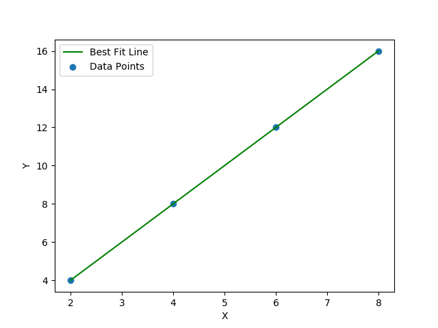
- The line for which the total prediction error is minimum is the Best Fit Line.
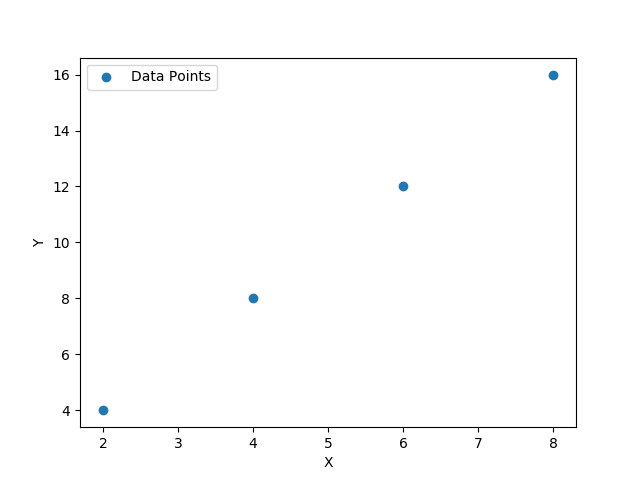
Data
Fit Line
Math
Let's get the math stuff out of the way first, shall we? Here's an equation we're all too familiar with :
$$\Large{y = m.x + c}$$
Where \(x\) is the independent variable, \(y\) is the dependent variable, \(m\) is the slope of the line and \(c\) is the \(y\)-intercept. Before diving into the ML way, a.k.a. Gradient Descent, here's the formula for finding \(m\) and \(c\).
$$\Large{m = \frac{\bar{x}.\bar{y} - \overline{x.y}}{(\bar{x})^2 - \overline{x^2}}} \hspace{10em} \Large{c = \bar{y} - m.\bar{x}}$$
Translate this into python and you're left with something that looks like :
import numpy as np

m = (np.mean(x_data) * np.mean(y_data) - np.mean(x_data * y_data)) /
					(np.mean(x_data) * np.mean(x_data) - np.mean(x_data * x_data))
c = np.mean(y_data) - m * np.mean(x_data)
Quite simple, moving on.
Getting Started
Let's create a few data points which we can use for visualization first.
import numpy as np
x_data = np.array([2, 4, 6, 8])
y_data = np.array([4, 8, 12, 16])
Use matplotlib to plot the points and display them.
import matplotlib.pyplot as plt
plt.scatter(x_data, y_data)
plt.show()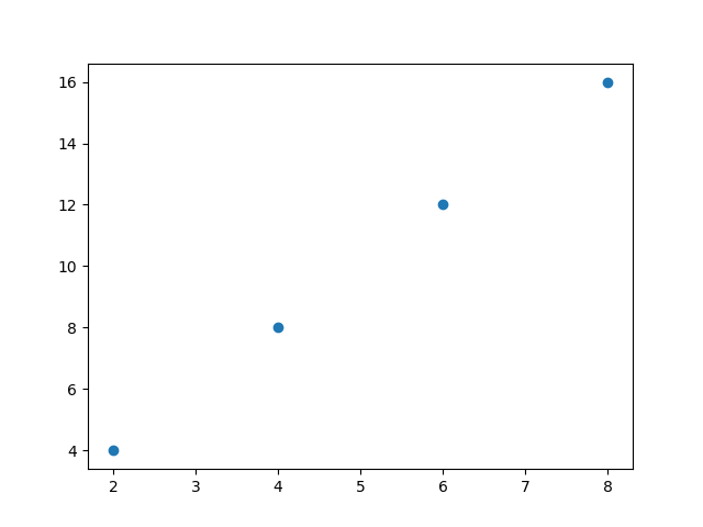
Time for Gradient Descent to step into the picture. It's an optimization technique used to find a local minima which minimizes a specific cost function. MSE would be the cost function in this situation and we need to find the values of \(m\) and \(c\) which will minimize it, giving us the best fit line. Here's a line that's not a great fit. The red lines indicate how wrong the prediction was for that specific data point. The distances are squared and summed up, giving us the squared error. The mean of this value is considered for minimization.
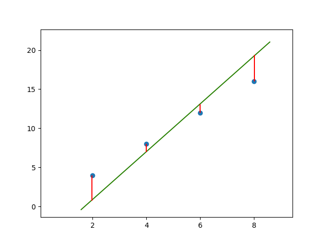
\(\hat{y}\) is the predicted value while \(y\) is the true value.
Imagine being on top of the hill, blindfolded. You need to get to the bottom of the hill, so you start moving in the direction which slopes downward. You take small steps and keep moving down the slope, till you eventually get to the bottom of the hill. There's no better analogy to explain how Gradient Descent works.
We can visualize the feature space in 3-D for the points that we just plotted using matplotlib.
from mpl_toolkits.mplot3d import Axes3D
mse = []
weight = []
bias = []
for w in np.arange(-10, 10, 0.5):
	for b in np.arange(-10, 10, 0.5):
		loss = 0
		for x_val, y_val in zip(x_data, y_data):
			y_pred = w * x_val + b 				# y = m * x + c
			loss += (y_pred - y_val) * (y_pred - y_val) 	# MSE Loss
		mse.append(np.mean(loss))
		weight.append(w)
		bias.append(b)

fig = plt.figure()
ax = plt.axes(projection = '3d')
ax.scatter(weight, bias, mse)
ax.set_zlabel('mse')
plt.show()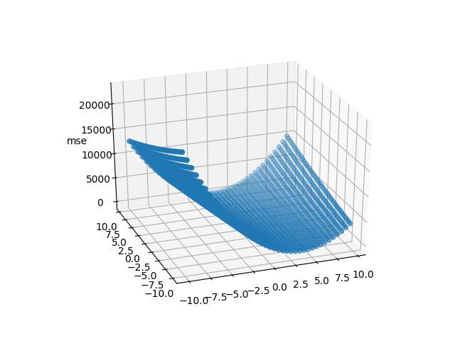
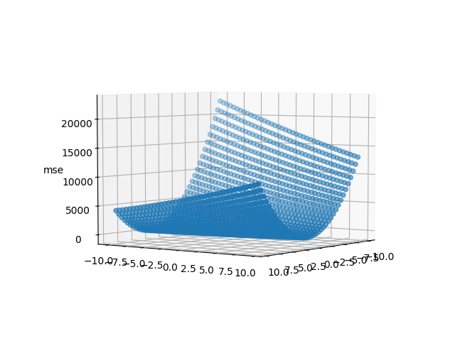
This 3-D figure is our imaginary hill. Say we started at the top of this hill. The current value of \(m\) and \(c\) is known to us, which can be used to calculate the MSE. Now, we need to figure out the direction in which we should take our step. To do this, we're going to calculate the slope/gradient at that point, which can be obtained by simple calculus (differentiation). The derivative of the the MSE is taken w.r.t. \(m\) and \(c\).
$$loss_i = (\hat{y_i} - y_i)^2 \hspace{10em} \hat{y_i} = m.x_i + c$$ $$loss_i = (m.x_i + c - y_i)^2 \hspace{13em}$$ $$\frac{dloss_i}{dm} = 2.x_i . (\hat{y_i} - y_i) \hspace{5em} \frac{dloss_i}{dc} = 2.(\hat{y_i} - y_i)$$
A positive gradient would mean that the hill is sloping upwards so a step in the opposite direction is needed. A negative gradient would mean that the hill is sloping downwards and we should step in that direction. Once we have the gradients, how do we take this 'step'?
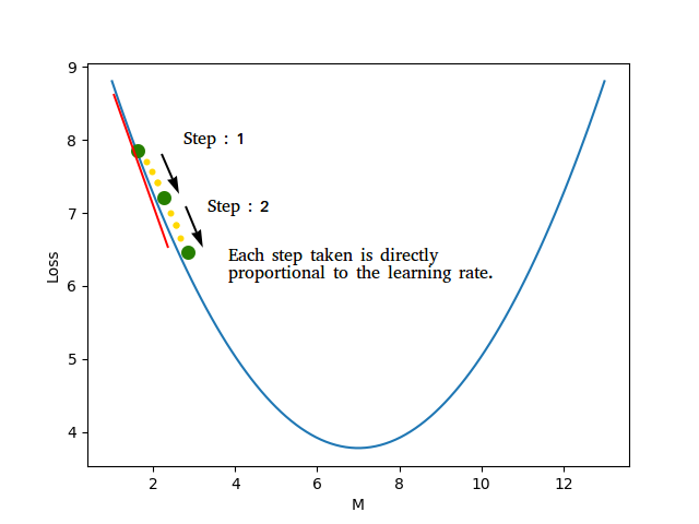
$$m = m - learning\_rate * gradient_m \hspace{10em} c = c - learning\_rate * gradient_c$$
The learning rate is an important term which signifies how big the step is. It's multiplied with the gradient and subtracted from \(m\) and \(c\) which ensures that we move in the right direction. It's easier to imagine in a 2D space. Let's pretend that \(c\) doesn't exist and the equation is \(y = m.x\) for the time being.
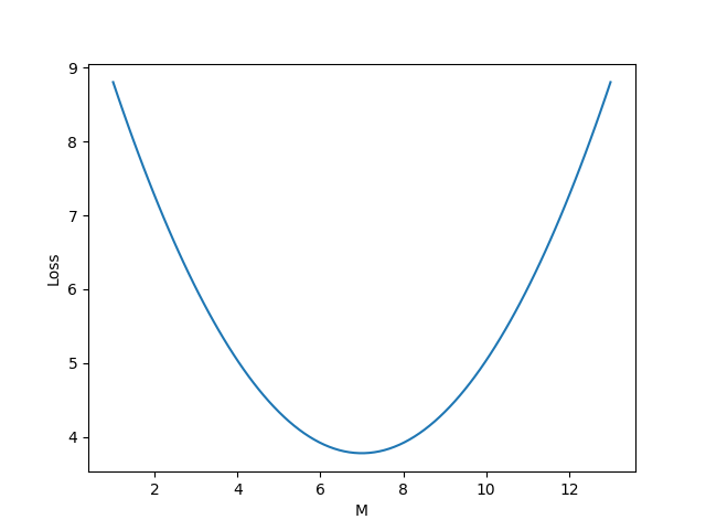
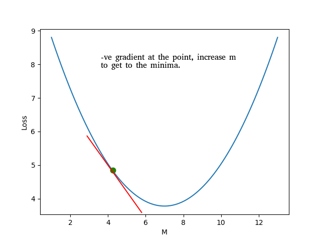
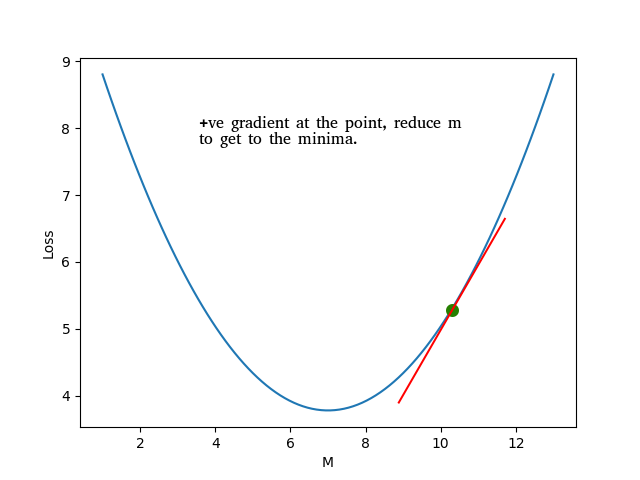
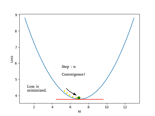
Using this formula \(m = m - learning\_rate * gradient_m\), we can see that a negative gradient would result in increasing \(m\) and a positive gradient would reduce \(m\). We also don't want to keep the learning rate too high because it might result in overshooting and completely missing the value of \(m\) for which the loss is minimum. But if the learning rate is too small, then it will take a long time for \(m\) to converge.
Good Learning Rate
And that's all you need to know before you can code it all from scratch. Let's dive right in!
We'll use the previously declared numpy arrays and move forward. First, we need to randomly initialize the values of \(m\) and \(c\). It can be anything, but we'll use \(1\) for now. We also need to initialize our learning rate and \(0.001\) is usually a good value.
m = 1
c = 1
lr = 0.001
Now, let's define a function which will return the value of \(\hat{y}\) along with our loss \((\hat{y} - y)^2\)
def forward(x):
	return m * x + c

def loss_fn(y_pred, y):
	return np.power(y_pred - y, 2)
We can move on to iterating over the data to train/update\(\thinspace\) \(m\) and \(c\). We'll update these values after calculating the loss for each data point, and we'll iterate over the data multiple times to make sure that we get the correct values of \(m\) and \(c\). Iterating over the entire data set once is called an epoch.
for epoch in range(100):
	for x_val, y_val in zip(x_data, y_data):
		y_pred = forward(x_val)
		loss = loss_fn(y_pred, y_val)
		grad_m = 2 * x_val * (y_pred - y_val)	# gradient for m
		grad_c = 2 * (y_pred - y_val)		# gradient for c
		m -= lr * grad_m			# update step for m
		c -= lr * grad_c			# update step for c
And we're done! All that's left is displaying the final values for \(m\) and \(c\), testing against some random values, and plotting the results.
x_test = np.array([10, 12, 14, 16])
print m, c
print [(m * x + c) for x in x_test]
line = [(m * x + c) for x in x_data]

plt.plot(x_data, line)
plt.show()
m:1.8867 c:1.015
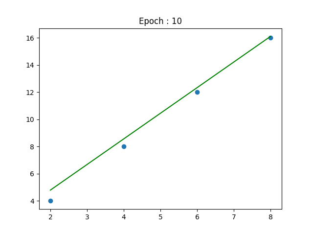
m:1.9999 c:0.000
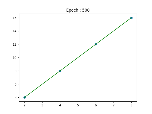
As you can see, the line keeps getting better with time. After a certain number of epochs, \(m\) and \(c\) converge to values which minimize the cost and we end up with the line of best fit! That's all there is to it. You have unknowingly built your first neural network, although it just consists of 1 neuron. The variables \(m\) and \(c\) are actually the \(weight (w)\) and \(bias (b)\) of a neuron in a neural network. But I'm going to leave that for another time.